Files: https://strutive07.github.io/assets/images/4_1_2_3_Decision_Boundary_introduction_to_logistic/IE661-Week_4-Part_1-icmoon-ver-1.pdf last update datetime: Jan 15, 2020 12:52 AM
나이브 베이즈에서는 naive assumption에 대해 정의가 필요했다. 이 navie assumption 정의를 하지 않는 logistic regression을 배워보자.
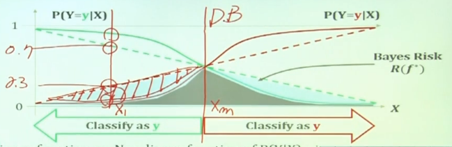
판단이 바뀌는 지점을 Decision boundary 라고 한다.
결국 decision boundary 근처에서 bayes risk를 줄여야 하므로, S curve 형태를 띄게 해야한다.
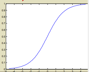
예시로 sigmoid function 이 있다.
Classification with one variable
하나의 variable로 decision boundary를 linear 하게 찾아보자.
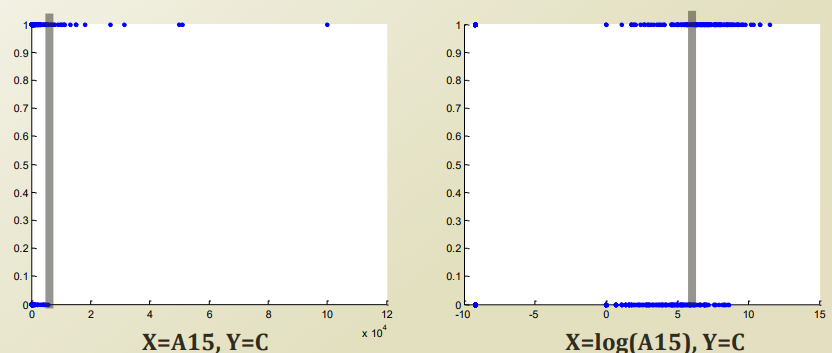
일반적으로 보았을떄 false 인 사건과 true인 사건이 linear 하게 나눠지지 않는다. x 값이 급격하게 커질경우 참으로 바뀌는 경향도 보인다.
값이 급격하게 커지는 것을 잘 학습하기 위해서 이 경향성을 해치지 않고, 값을 누그러뜨릴 수 있다.
log 를 취하는것이다. log 는 monothonic 하게 증가하므로 경향성이 바뀌지않고 값으 범위만 바뀔 수 있다.
Linear function vs non-linear function
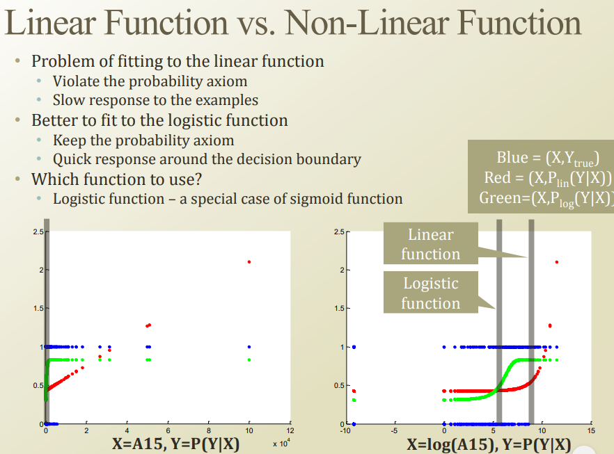
데이터가 discrete 한 상태에서는 linear regression을 사용하면 안되지만, 전에 배웠던 것이므로 한번 예시로 돌려보자.
파랑색: 정답
초록색: logistic regression
빨강색: linear regression
빨강색의 경우, 총 확률이 1인데 1을 넘어가는 에러가 발생하고있다.
당연히, 값이 높은 사람들이 true, 값이 낮은 사람들이 false 인 경향이 많기 때문이다.
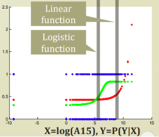
log 를 씌워서 decision boundary를 보자. 확실히 logistic regression이 bayes risk가 적은것을 알 수 있다.
Logistic function
Sigmoid function
- Bounded
- y값이 -1 ~ 1 로 제한되어있음.
- differentiable
- 부드러운 s 커브 형태
- real function
- defined for all real inputs
- -무한 ~ 무한 까지 정의되어있음
- with positive derivative
- 단조증가
종류들
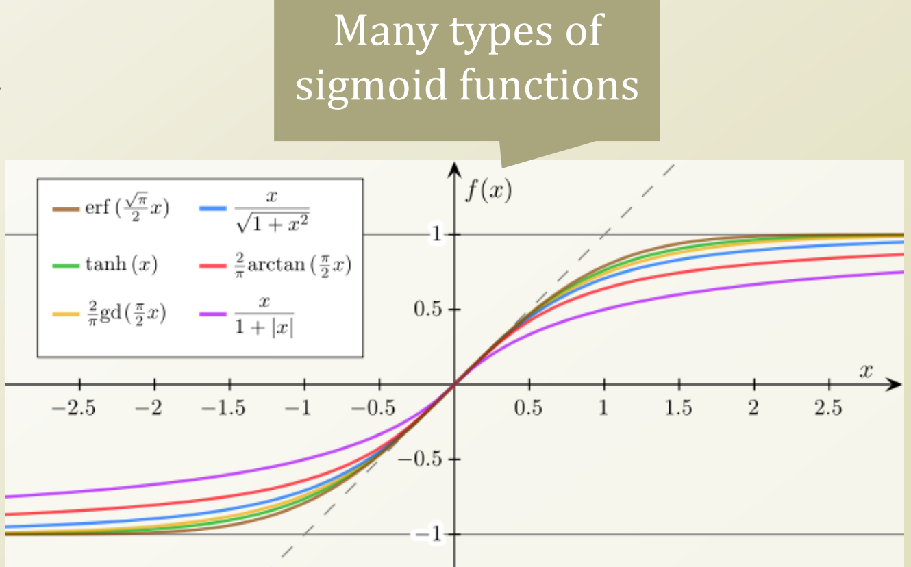
- tanh, arctan 등은 뉴럴 네트워크에서 많이 사용됨.
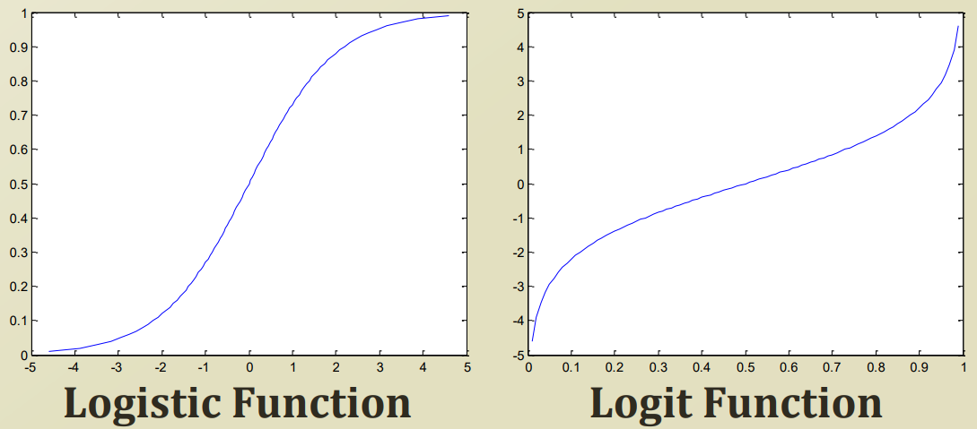
logistic function의 역함수가 logit function 이다.
logistic function
logit function
sigmoid function들은 미분하기 쉬움.
Logistic function fitting
우리 데이터에 대해 logistic function을 fitting 시켜보자.
기존 logit function을 사용하는 이유는, logit function은 x 가 0~1인 반면, logistic function은 그 역함수인 y가 0~1이다.
우리는 logit function의 결과와 x 값이 동일해지는것을 원하므로, logit function을 사용할것이다,.
여기서 logit function의 입력 값은 확률값이다.
특정 데이터 X 가 있고, 이 데이터를 linear shift를 해서 logit function을 이동시키거나 weight를 곱하여 형태를 변형시켜야한다. 여기서 weight 와 bias 를 구하는 작업을 fitting이라고 한다.

이를 linear regression에서 했던것처럼 행렬로 일반화하면 다음과같이 쓸 수 있다.
이제 우리는 theta를 구하면 특정 사건일때 확률 P 를 구할 수 있을것이다!
| 여기서 다시 linear regression을 생각해보자. 우리가 구하고자 하는 X theta 는 결국 P(Y | X) 를 구하는것이다. |
why?
X 가 주어졌을떄, 각 class 의 확률이 어떻게 주어질것인가? 이므로.
이를 동일하게 logistic regression에 대입하면된다!
logistic regression은 확률이 log 안에 존재하므로 다음과같이 표현된다.
위에서 계속 언급했다싶이, logistic function 과 logit function은 역함수관계이다. 이를 사용해서 위 함수를 풀어보면 다음과같은 꼴이 완성된다.
binary classification 이라고 예를 들어보자.
자! 그래서 우리는 theta만 알아내면 된다는것을 찾았다.
여기서 확률값이 logistic function을 따른다 하면, 다음과같이 나타낼 수있다.
Finding the paremter, θ
Maximum conditional likelihood estimation
MLE 와 동일하게 class variable Y 를 구하는것은 동일하지만, input feature X 를 고려하여 구하는것이다.
MLE때 했던 내용이니 log로 변환하는 과정은 생략.
생각하기 쉽게 binary classificaiton 이라고 생각해보자.
| 그러면 우리는 P(Y | X) 가 베르누이 분포를 따를것이라는것을 알 수 있다. |
여기에 로그를 취해보자.
여기서 아래 부분은 어디서 많이 본것이다. 바로 logistic regression에서 구했던 식이다!
이걸 그대로 식에 대입해보자.
Partial derivative to find a certain element in θ
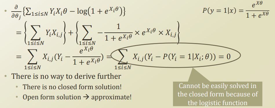
최종 형태가 theta = blabla 형태로 떨어지지 않는다.
따라서 계산하기가 쉽지않다.
따라서 theta를 구하려면 저 식을 근사해서 theta를 구해야한다.
그럼 어떻게 approximation 할 수 있을까? 다음 강의에서 이어서…