Create time: Feb 09, 2020 12:24 PM Update time: Feb 11, 2020 9:13 PM
Convex function 은 위와같은 형태를 가진다.
minimize, maximize 해야하는 objective function 이 있고, 여기에 inequality constraint, equality constraint 가 있다.
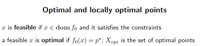
objective function, inequality constraint, equality constraint 을 모두 만족하는 domain x 가존재한다면, 이를 fessible 하다 라고 부른다.

하나라도 벗어난다면, 이는 fessible 하지 않다는것이다.
fessible set 인 domain x 를 objective function 에 적용하였을 경우, 최솟값이 존재하는 경우, 이를 optimal point라고 부른다.
fessible set이라고 해서, 무조건 optimal point가 있는것은 아니다. 위 필기 참조.

domain 에 제한을 걸어둔 상태에서 optimal value가 존재한다면, 이는 locally optimal point 이다.
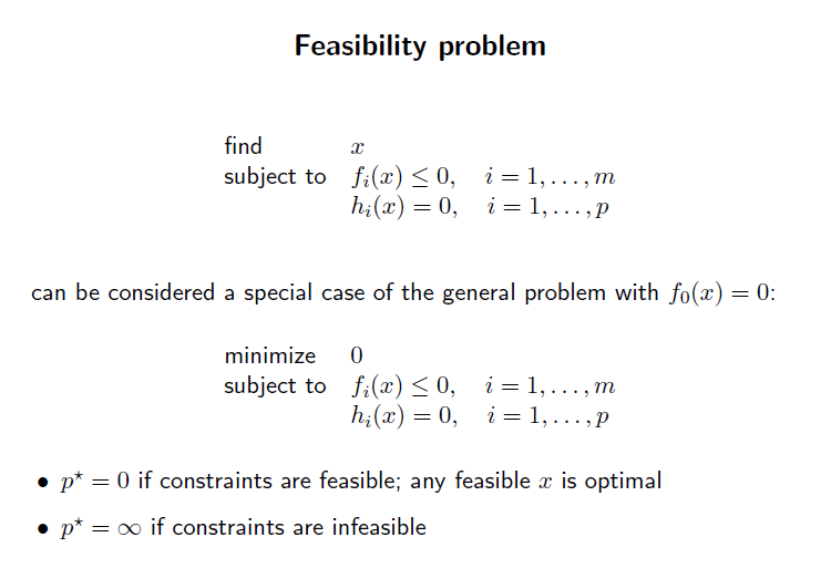
만약 objective function 이 identically zero 라면, optimal value 는 0 또는 양의 무한 일것이다. 이때 0일때는 feasible set 이 non-emtpy, 양의 무한대 라면 feasible set이 emtpy 라는것이다.
우리는 이런것을 feasible problem 이라고 부른다.
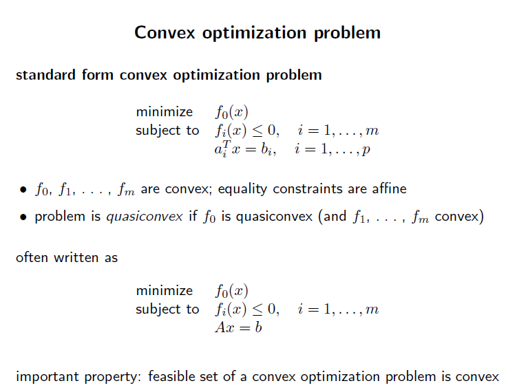
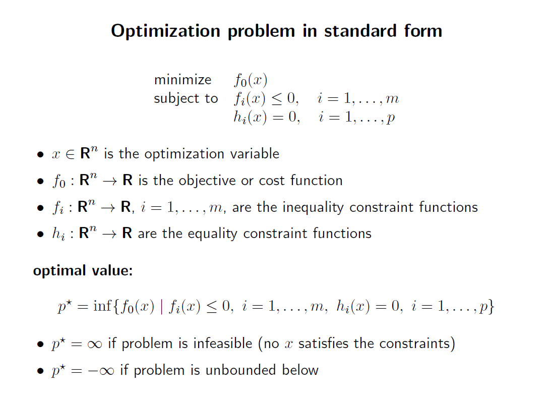
Convex optimization problem의 standard form은 위와같다. standard form에서는 inequality constraint 오른쪽 항에 무조건 0이 와야한다.
그리고 equality constraint는 affine function 형태 이다.

중요한 특징으로, convex optimization problem 의 fesible set은 convex 하다.
standard form 은 그 형태가 변하면 안됨.
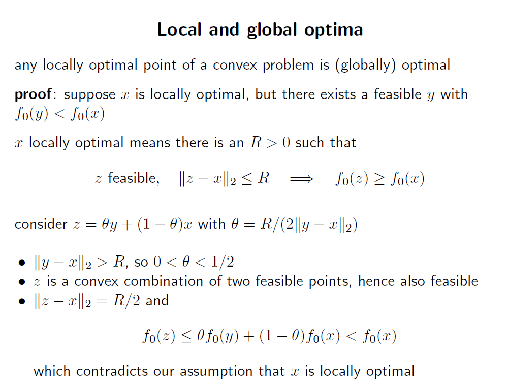
Convex problem에서 local optimal point 는 global optimal point 이다.
Proof:
x 가 locally optimal 인데, fessible y 중 f0(y) < f0(x) 이 존재한다면, y 와 x 의 convex ccombination set 중 하나의 점, z 에 대하여 다음 식을 만족해야함.

위는 모순이므로 locally optimal point x 는 global optimal point 이다.
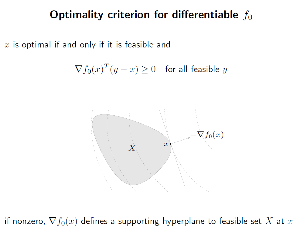
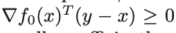
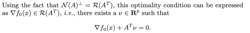
first-order condition for optimality 는, convex problem 에서 objective function f 가 미분 가능할 때, 아래의 부등식은 optimal point x 에 대한 필요충분 조건이 된다.
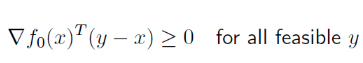
이는, 미분값이 0이 아닌 경우에서 위 수식이 0이 되는 지점을 support vector 로 삼음 support hyperplane이 만들어짐을 의미한다. 이때 support hyperplane의 방향은 -미분값 이다.
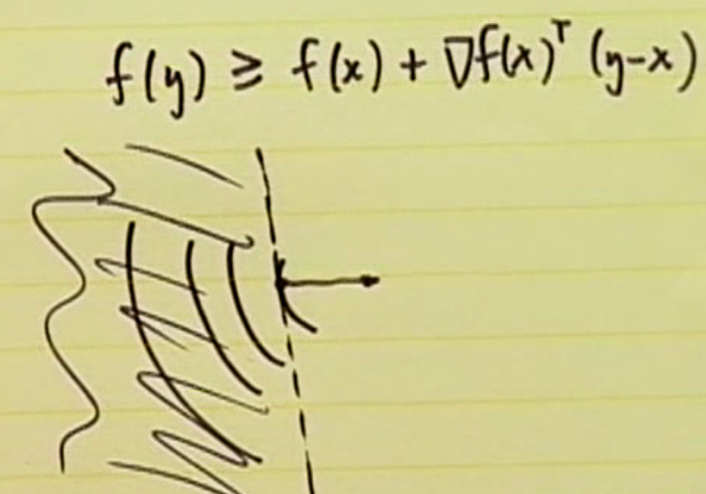
모든 y에 대해서, 위 수식을 만족한다면, y 가 속해있는 set C 는 -미분값 의 반대방향 의 hyperplane 에 포함된다는것이므로, x 는 optimal point가 된다.
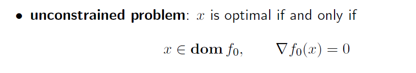
예시를 살펴보자. unconstrained 이라면, 미분값이 0이 되는 부분이 global optimal이 될것이다.
proof:
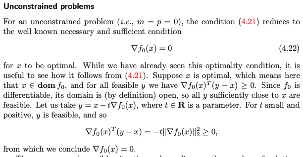
만약 x 가 optimal point 라면, 모든 feasible y 에 대하여 아래 수식을 만족해야함.
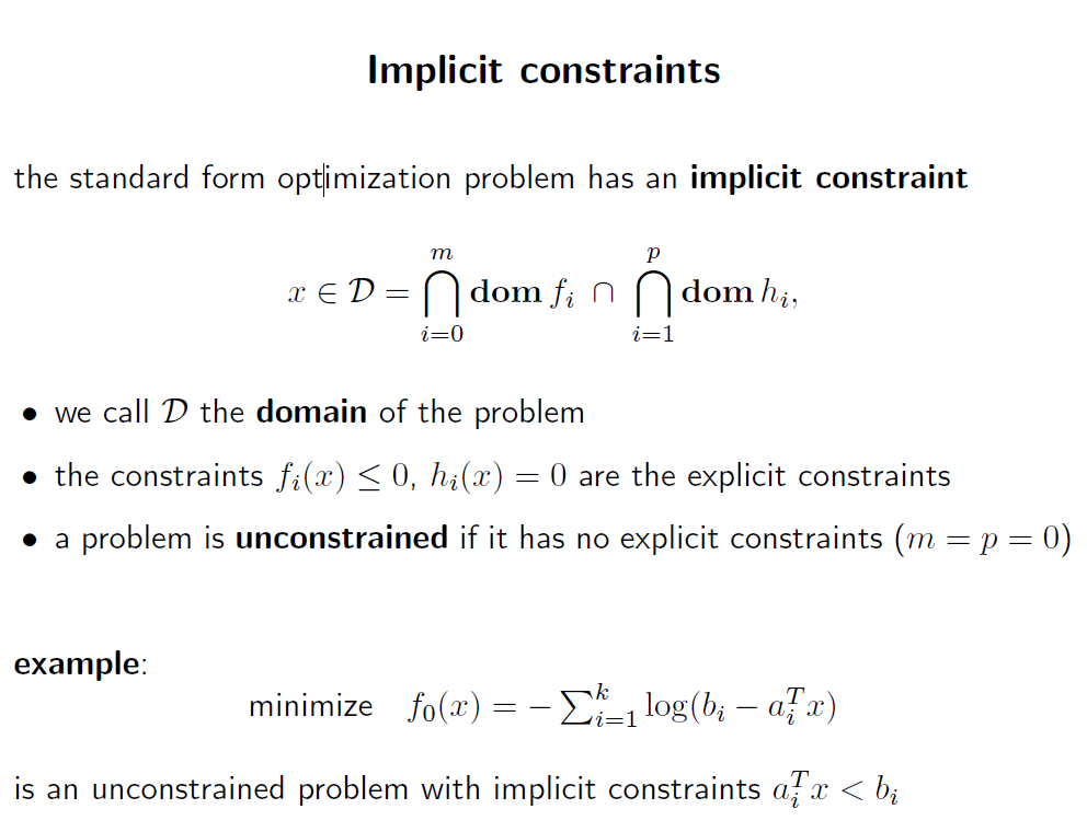
f0가 미분가능하다면, domain은 open 되어있다.
y가 충분히 큰 경우에는 무조건 0보다 크고, y가 x에 가까울 때를 가정해보자.
위와같이 가정하였을때, 위 식을 만족하는것은 미분값이 0이 될 때 뿐이다. 따라서 unconstrained problem에서 optimal point 은 미분값이 0이 되는 지점이다.
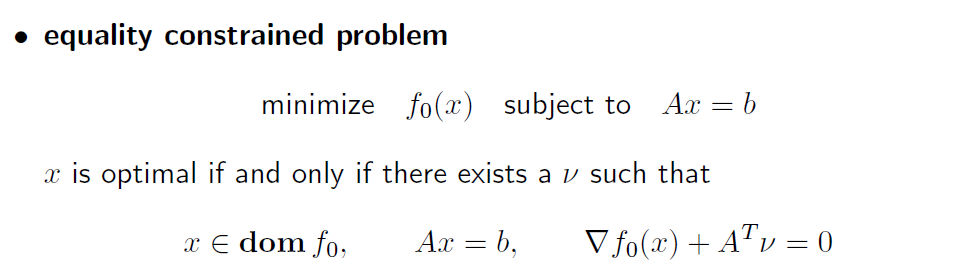
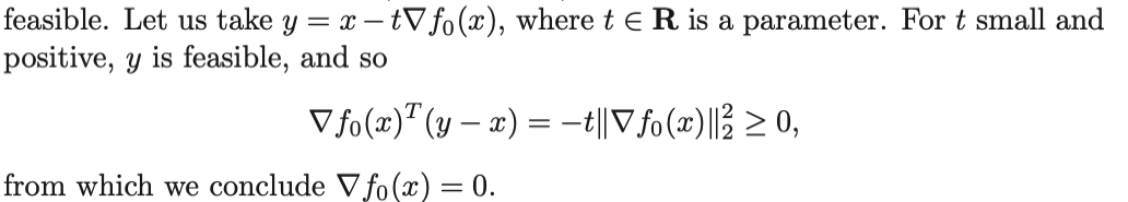
equality constrainted problem. 이 문제의 feasible set 은 affine 이다.
증명
y - x = z 라고 치환해보자.
그럼 위 2번째 식 처럼 표현할 수 있다.
위 linear function 이 subspace 에서 non-negative 한다면, 이는 subspace위에서 0 이여야 함. 이는 두 vector 가 식 3 번 처럼 othogonal 관계여야함.
이를 위와같이 치환해서 생각할 수 있음.
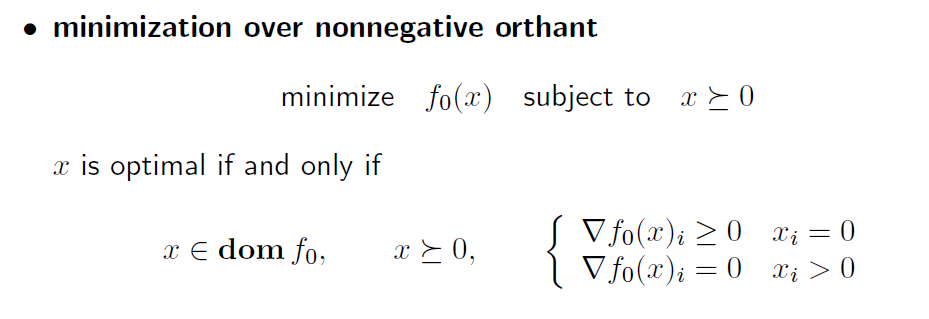
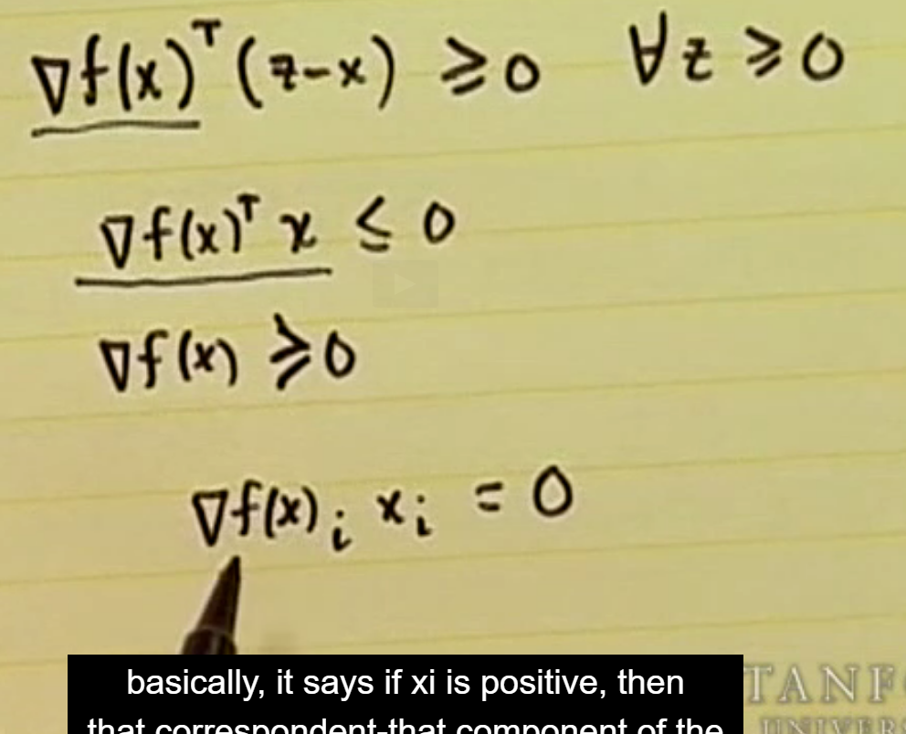
non-negativity constraints 를 가지고 있는 문제의 예시.
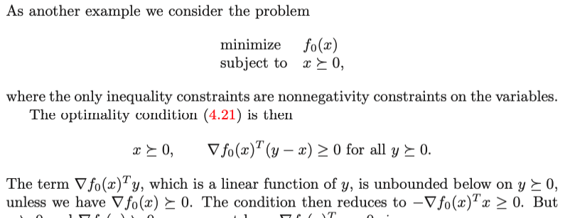
convex problem이므로, 미분값이 공간 위에서 0보다 크거나 같고, y가 0보다 크거나 같다면, y 항은 항상 양수이므로 비교에서 빠질 수 있다.
그럼 문제는 위 마지막 줄의 마지막 수식처럼 x term만으로 표현할 수 있다.
그런데 x 가 0보다 큰 상황에서 위 수식을 만족하려면, 미분값은 무조건 0 이여야 함.
아래 필기 참조.
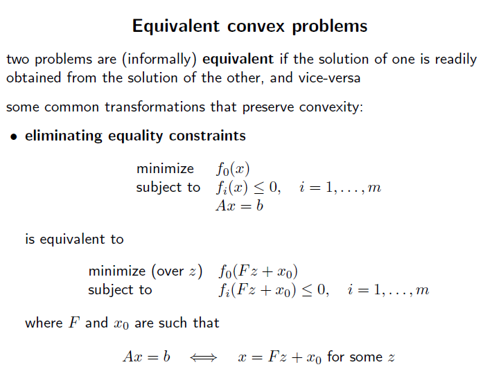
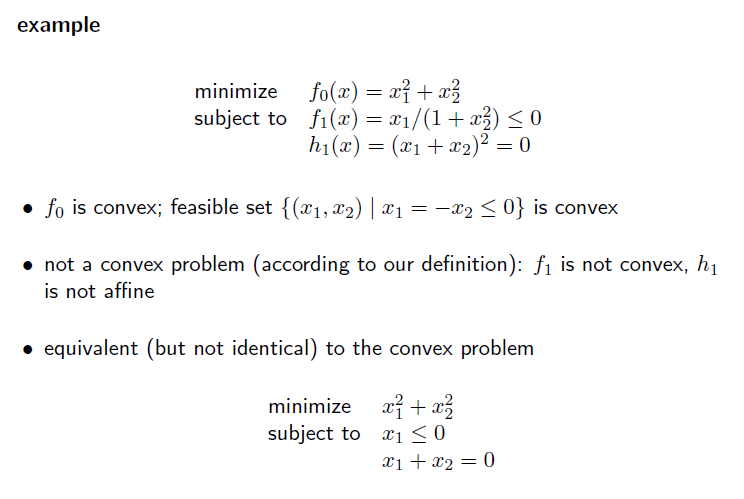
Convex optimization problem에서 내부 수식을 변형하면서도 그 convexity를 잃지 않도록 하는 연산들을 알아보자.
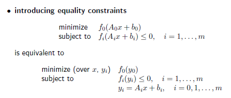
내부 식을 하나의 affine function 으로 생각하고, 이를 하나의 변수로 치환한다. 이때 변환된 함수는 equality constraint로 추가된다.
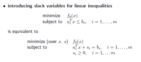
inequality constraint를 slack variable을 추가하여 하나의 equality constraint와 slack variable만 있는 inequality constraint로 치환한다.
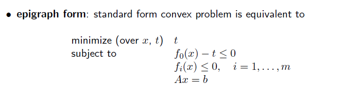
만약 objective function 이 linear function 이고, 새로운 constraint function f(x) - t 이 convex functinon 이면, epigraph form 의 problem 또한 convex 하다.
아래 그림처럼, t를 아무리 변경하여도 global optimal 이 변하지 않는것을 알 수 있다.
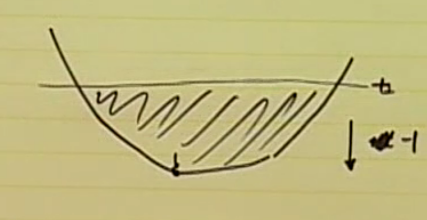
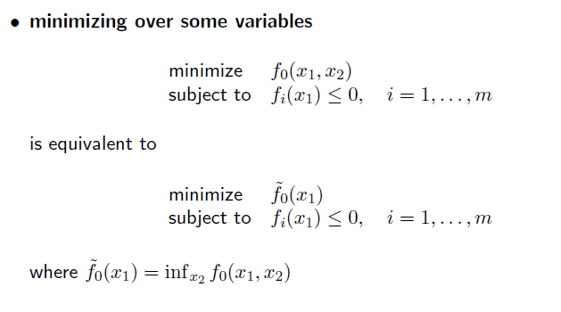
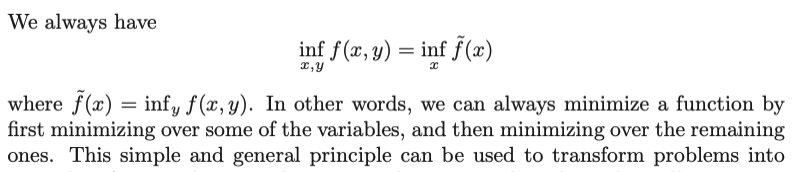
inf 는 하나의 variable씩 진행할 수 있음. 이를 이용하여 위 수식은 전개할 수 있음.
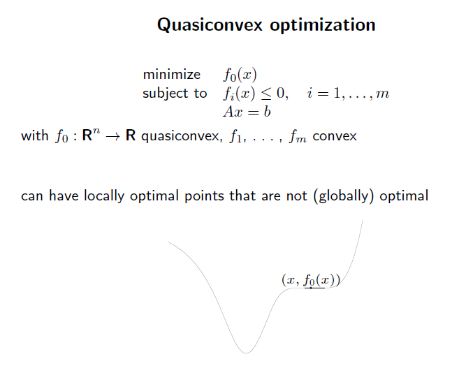
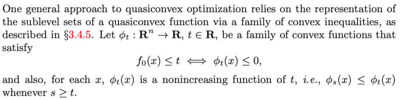
quasiconvex optimization. 은 objective function이 quasiconvex function이고, constraint function이 convex function인 optimization problem이다.
quasiconvex optimization의 local optimal point는 무조건 global optimal point인것은 아니다. 기하학적으로 생각하면, 위 그림처럼 saddle point가 있을 수 있음.
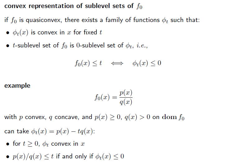
objective function 을 sublevel set 의 표현으로 바꿔보자.
non-increasing이라면, sublevel set 을 구성하는 알파의 값이 클수록 optimal value는 작거나 같을것이다.
위 성질을 이용하여 global optimal value를 구해보자.
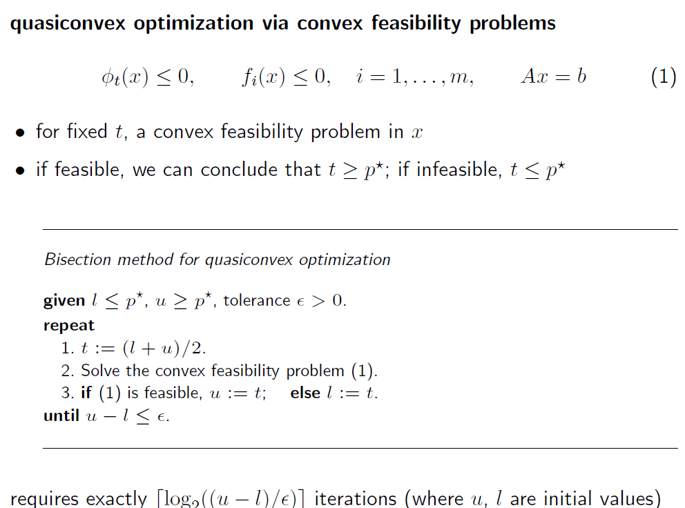
quasiconvex optimization을 binary search 문제로 치환해서 풀어보자.
upperbound, lower bound를 받고, 이 안에서 optimal value를 찾는것이다. binary search를 하면 log 시간 안에그 안에서 존재하는 local optimal value를 찾을 수 있을것이다. upper bound, lower bound를 잘 설정하면 global optimal value 를 찾을 수 있을것이다.
Linear programming
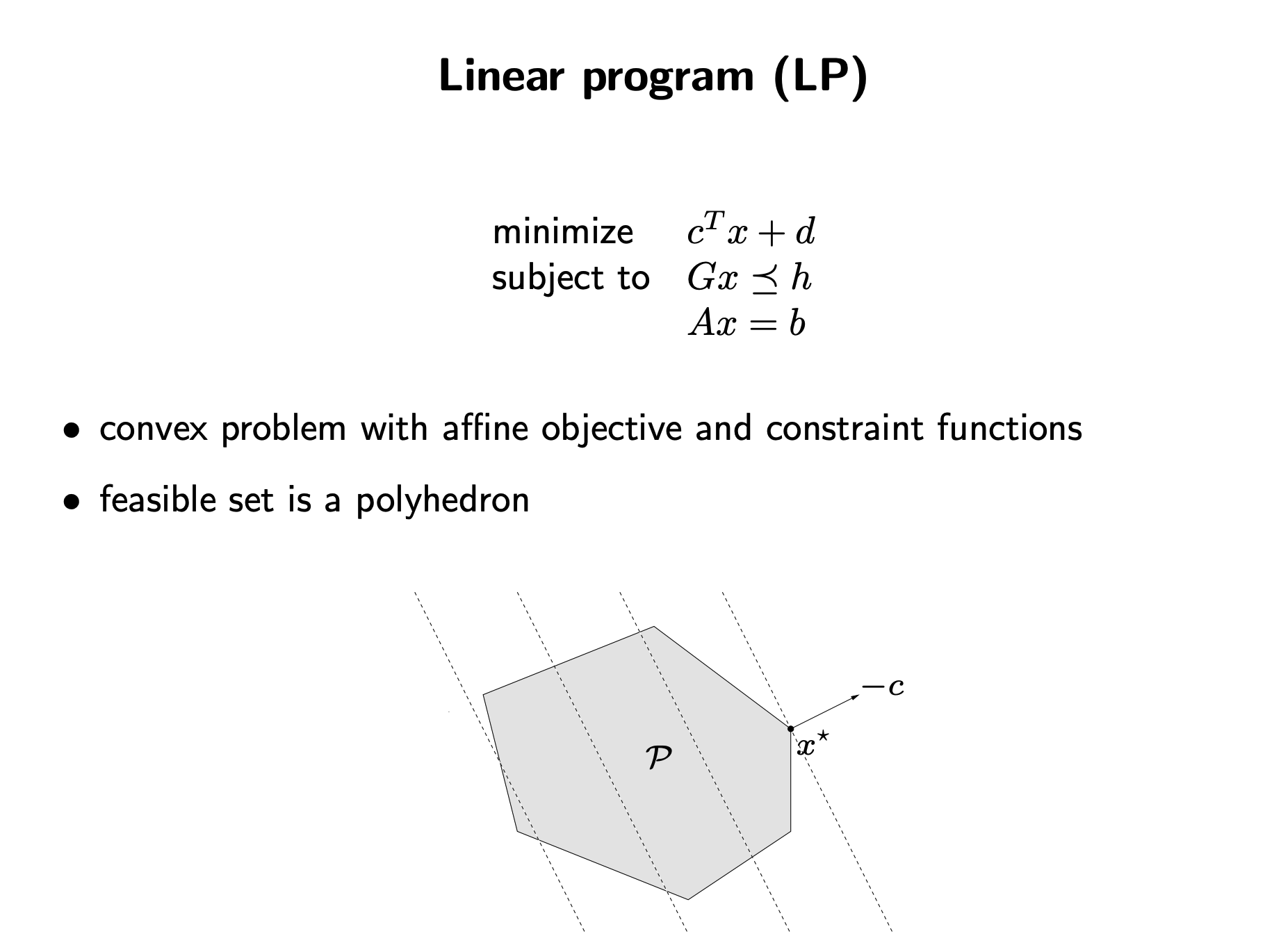
Linear programming은, convex optimization의 한 종류로, objective function 과 constraint function 모두 affine function 으로 이루어진 problem 이다.
기하학적으로 생각해보면, polyhedron 형태의 feasible set 에서 affine function 하나를 minimize 하는것이고, 결국 특정 위치에서의 support hyperplane을 찾는 형태가 될것이다.
이때 feasible set은 polyhedron 형태로 나타내 질 수 있다.
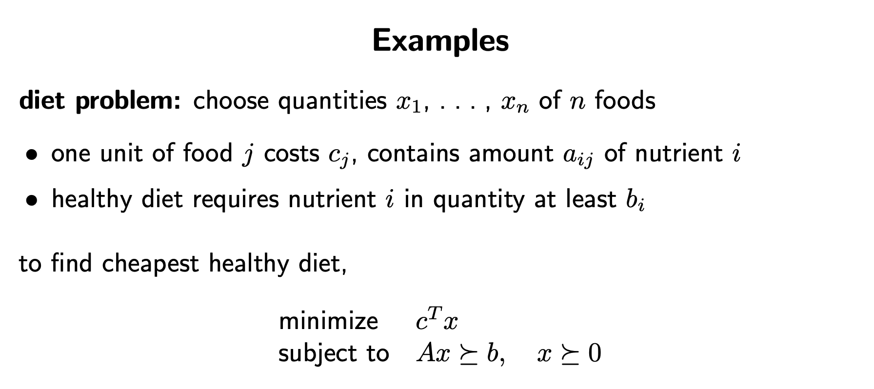
대표적인 예시 몇가지를 살펴보자.
diet problem 이 있다고 가정해보자. variable x 는 음식의 종류, c 는 각 음식에 대한 cost, a 는 각 음식이 가지고 있는 영양정보라고 해보자.
constraint function은 각각의 영양소의 최소 섭취 양이 정해져있다.
이를 위의 LP 형태로 나타낼 수 있다. constraint function을 (AMOUNT * 양) ≥ 최소 기준 을 만족하도록.
여기서 최적화 하는 objective function 은 최종 cost 이다.
조금 더 수학적인 예시를 살펴보자.
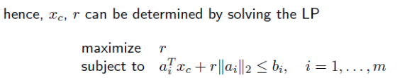
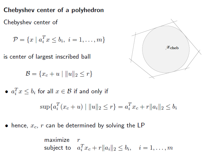
chebyshev center of a polyhedron 이라는 문제 이다. polyhedron 내부에서 생성될 수 있는 가장 큰 원을 찾는것이다.
문득 보면 quadratic programming 같이 보이지만, LP 이다.
ball 을 중심에서 반지름의 거리 보다 작거나 같게 떨어진 공간을 의미해보자.
그리고 중심이 b 안에 있어야 한다고 해보자. 각 b 를 합치면 polyhedron이 될것이다.
이 두 식을 합치면 아래와 같이 만들어진다.
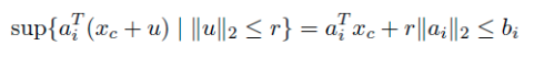
위 식이 constraint function 이 되고, objective function 은 반지름 r 을 최대화 하는것이다. 중심 x_c는 여러개 있어도 상관 없다.